RNA-Seq
RNA-Seq
泡泡RNA-Seq指南
RNA-Seq参考
根据基因组进行量化
RNA-Seq根据基因组进行量化时,参考数据是基因组序列,基因组注释文件是基因组的注释信息,包括基因的位置、外显子的位置、基因的功能等信息。该方法将对齐文件与注释相交叉,以产生“计数”,然后过滤这些计数以保留统计上显著的结果。定量矩阵代表对齐与标记为转录本一部分的区间重叠(交集)的次数。
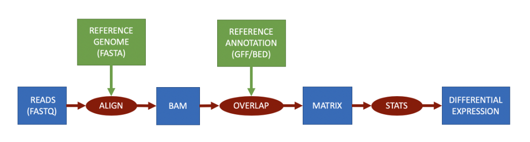
在通过参考基因组和注释信息对读段进行映射,然后再进行表达量估算时候,又有两种不同的基因表达量分析方法。
- 基因水平分析:
- 这种分析方法把一个基因的所有转录本(即由基因的不同区域(外显子)组成的不同版本)视为一个整体。
- 在这种分析中,不区分各个不同的转录本,而是将它们合并为一个单一的序列,这个序列包括了该基因的所有外显子。
- 这个合并的序列被认为是“代表性”的,但它可能并不对应于任何实际存在的单一转录本,它更像是一个虚拟的总和。
- 对于某些研究目的而言,这种简化的方法足够用来获取有意义的数据,尤其是当研究的重点是基因整体活动水平时。
- 转录本水平分析:
- 与基因水平分析不同,转录本水平分析关注于每个单独的转录本。
- 这种方法不会将不同的转录本合并,而是独立地测量每一个转录本的表达量。
- 这允许研究者观察到基因内部异构体(即同一基因的不同转录本版本)的丰度变化,这些变化可能对细胞功能和调控至关重要。
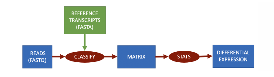
根据转录组进行分类
RNA-Seq根据转录组进行量化时,参考数据将是每个转录本的 FASTA 文件。分类将把每个读取分配给一个转录本,从而解决过程中的歧义。每个转录本的量化矩阵将表示读取被归类为该特定转录本的次数。
目前主流的能够实现基于分类的RNA-Seq工作的软件有:
- Salmon
- Kallisto
我们也能从参考基因组及注释文件中使用gffread工具生成转录组的FASTA文件。1
2
3
4conda install gffread
# Extract the transcripts.
gffread -w refs/transcripts.fa -g refs/22.fa refs/22.gtf
参考基因组
通常情况下,当我们下载一个参考基因组后,我们需要知道一些基本信息,比如基因组的大小、基因组的组成、基因组的注释信息等。这些信息对于我们后续的分析非常重要。
参考基因组大小
1 | seqkit stats *.fa |
输出:1
2file format type num_seqs sum_len min_len avg_len max_len
genomic.fa FASTA DNA 194 3,099,750,718 970 15,978,096.5 248,956,422
有194个序列(染色体+特定基因组序列标识符),总长度为3,099,750,718bp,最短序列为970bp,最长序列为248,956,422bp,平均序列长度为15,978,096.5bp。
有多少个染色体
1 | cat *.fa | grep ">" |
每个染色体的长度
可通过samtools faidx命令获取每个染色体的长度。1
2samtools faidx *.fa
cat *.fa.fai
输出:1
2
3
4
5
6
7
8
9
10
11
121 248956422 56 60 61
10 133797422 253105810 60 61
11 135086622 389133248 60 61
12 133275309 526471372 60 61
13 114364328 661967995 60 61
14 107043718 778238454 60 61
15 101991189 887066292 60 61
16 90338345 990757392 60 61
17 83257441 1082601434 60 61
18 80373285 1167246557 60 61
···
···
第一行:染色体名称。第二行:染色体长度,表示这个染色体的总长度。第三行:染色体的偏移量,这是染色体序列在FASTA文件中的起始字节位置。这意味着,如果你想定位到第10号染色体的序列开头,你需要从文件的开头跳过253,105,810个字节。第四行:每行序列的长度,60,这表示在FASTA文件中,每行表示的序列的字符数是60。这不包括行末的换行符。第五行:每行的长度,61,这个数字比序列的长度多1,说明每行的结束包括了一个换行符(通常是\n),所以每行的实际长度是61个字符。
参考基因组注释文件
参考基因组常见的注释文件格式有GTF(Gene Transfer Format)和 GFF(General Feature Format),两者都是文本格式的文件。这些文件包括了基因组上各种遗传标记的详细信息。
在RNA-Seq分析中,基因和转录本的注释通常是最核心的信息,因为它们直接关系到后续分析中的表达量计算和差异表达分析。基因级别的注释可以提供关于哪些基因在样本中被表达的信息,而转录本级别的注释则可以提供更细致的信息,比如不同的剪接变体。
然而,是否只需要基因和转录本的遗传标记信息取决于分析的具体目的:
基因表达定量: 如果只需要进行基因水平的表达量分析,那么基因的注释信息可能就足够了。
转录本表达定量和剪接分析: 如果要进行转录本水平的表达分析或者分析剪接变异,就必须要有转录本以及外显子的详细注释信息。
蛋白质编码分析: 如果分析涉及到蛋白质编码区域,例如寻找可能影响蛋白质结构的突变,那么编码序列(CDS)注释就很重要。
UTR区域分析: 对于研究转录后调控,比如microRNA的靶向等,5’ UTR和3’ UTR的信息会很关键。
调控元件分析: 如果研究的重点是基因的调控机制,那么启动子、增强子等调控元件的注释就显得非常重要。
1 | cat *.gtf | grep -v "#" | cut -f3 | sort | uniq -c |
CDS (Coding Sequence): 编码序列是指基因组中编码蛋白质的部分,这个数字(746300)告诉我们在注释文件中有这么多的编码序列条目。
Selenocysteine: 一种被称为“第21个氨基酸”的罕见氨基酸,它直接参与蛋白质的合成。这个数字(120)表明在注释文件中有120个编码selenocysteine的位点。
Exon: 外显子是成熟mRNA中保留下来的那部分DNA序列,可以转录并翻译成蛋白质。这个数字(1261907)表示注释文件中有这么多外显子。
Five_prime_utr (5’ UTR): 5’非翻译区(Untranslated Region)是位于起始密码子之前的mRNA序列部分,它不编码蛋白质,但有助于调控翻译过程。这个数字(149893)表示文件中有这么多的5’ UTR条目。
Gene: 基因是遗传的基本物理和功能单位,通常包含编码一个或多个蛋白质的序列。这个数字(58676)表示文件中有这么多基因。
Start_codon: 起始密码子是一段特定的核苷酸序列,它在mRNA上标志着蛋白质合成的开始。这个数字(86423)显示了有这么多的起始密码子被注释。
Stop_codon: 终止密码子是信号蛋白质合成结束的三个核苷酸序列之一。这个数字(78536)表示有这么多的终止密码子。
Three_prime_utr (3’ UTR): 3’非翻译区(Untranslated Region)是位于终止密码子之后的mRNA序列部分,它同样不编码蛋白质,但含有调控mRNA稳定性和翻译效率的重要元素。这个数字(148456)表示文件中有这么多的3’ UTR条目。
Transcript: 转录物是指DNA序列通过转录过程生成的RNA副本,在这里特指那些最终会被翻译成蛋白质或者具有其他功能的RNA分子。这个数字(206534)表明有这么多的转录物记录在注释文件中。
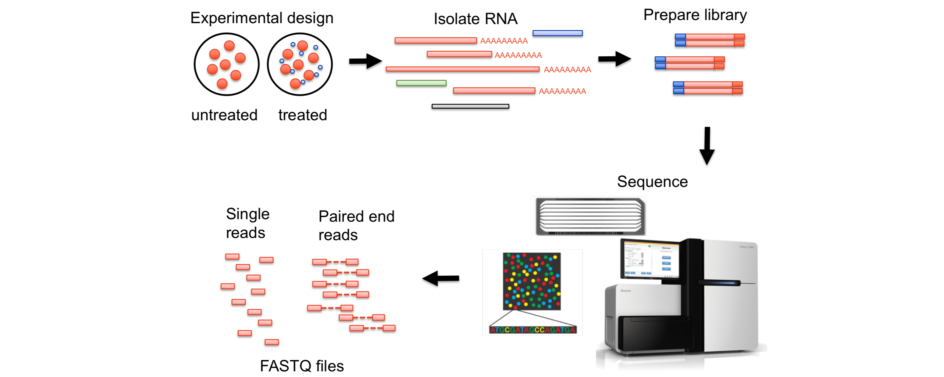
了解数据
通常情况下RNA-Seq数据是由fastq文件组成,fastq文件包含了测序仪输出的原始测序数据,每个fastq文件包含了大量的reads,每个read都是一个碱基序列,同时还包含了测序质量信息。我们可以通过查看统计fastq文件来获取数据的一些信息。
1 | # 统计fastq文件 |
输出:1
2
3
4
5
6
7
8file format type num_seqs sum_len min_len avg_len max_len
chip_HA_1_1.fq FASTQ DNA 40,478,593 2,023,929,650 50 50 50
chip_HA_2_1.fq FASTQ DNA 37,248,768 1,862,438,400 50 50 50
chip_HA_3_1.fq FASTQ DNA 28,160,024 1,408,001,200 50 50 50
chip_input_1_1.fq FASTQ DNA 42,065,898 2,103,294,900 50 50 50
chip_plau_1_1.fq FASTQ DNA 31,915,339 1,595,766,950 50 50 50
chip_plau_2_1.fq FASTQ DNA 43,102,269 2,155,113,450 50 50 50
chip_plau_3_1.fq FASTQ DNA 38,000,000 1,900,000,000 50 50 50
比对
构建索引
当我们将数据和参考基因组进行比对时,首先需要准备参考基因组的索引文件,不同的参考基因组比对工具需要不同的索引文件,比如STAR需要的索引文件是STAR_index,而HISAT2需要的索引文件是HISAT2_index。
以Hisat2为例,我们可以通过以下命令构建索引文件:1
2
3
4
5
6
7
8
9
10
11
12
13
14# The reference genome.
REF=refs/*.fa
GTF=refs/*.gtf
# Build the genome index.
IDX=refs/genome
hisat2_extract_splice_sites.py ${GTF} > ${IDX}.ss
hisat2_extract_exons.py ${GTF} > ${IDX}.exon
hisat2-build -p 16 --exon ${IDX}.exon --ss ${IDX}.ss ${REF} ${REF}
# Index the reference genome with samtools.
samtools faidx ${REF}
比对
1 | # Create the include sample list file. |
双端比对信息解读:1
2
3
4
5
6
7
8
9
10
11
12
13
1410000 reads; of these:
10000 (100.00%) were paired; of these:
650 (6.50%) aligned concordantly 0 times
8823 (88.23%) aligned concordantly exactly 1 time
527 (5.27%) aligned concordantly >1 times
----
650 pairs aligned concordantly 0 times; of these:
34 (5.23%) aligned discordantly 1 time
----
616 pairs aligned 0 times concordantly or discordantly; of these:
1232 mates make up the pairs; of these:
660 (53.57%) aligned 0 times
571 (46.35%) aligned exactly 1 time
1 (0.08%) aligned >1 times
10000 reads; of these: 10000 (100.00%) were paired: 总共有10000个读段,所有这些读段都是成对的,意味着每个读段都有相应的配对读段。
650 (6.50%) aligned concordantly 0 times: 有650对读段(占6.50%)没有一起成功比对到参考序列上。”一致比对”(concordantly)意味着两个读段以预期的相对方向和距离成功地比对到参考序列的同一个区域。
8823 (88.23%) aligned concordantly exactly 1 time: 有8823对读段(占88.23%)一致地比对到参考序列的唯一位置一次。
527 (5.27%) aligned concordantly >1 times: 有527对读段(占5.27%)一致地比对到参考序列的多个位置。
接下来的部分提供了关于没有一致比对的读段的更多细节:
- 650 pairs aligned concordantly 0 times; of these:
34 (5.23%) aligned discordantly 1 time: 在没有一致比对的650对读段中,有34对(占5.23%)以不一致的方式比对了一次。”不一致比对”(discordantly)意味着这些读段没有按照预期的相对方向或距离比对到参考序列的同一个区域,但仍然在某处找到了比对位置。
616 pairs aligned 0 times concordantly or discordantly; of these:
- 1232 mates make up the pairs; of these:
- 660 (53.57%) aligned 0 times: 在这616对既没有一致比对也没有不一致比对的读段中,总共有1232个单独的读段,其中660个(占53.57%)没有比对到参考序列。
- 571 (46.35%) aligned exactly 1 time: 有571个读段(占46.35%)比对到了参考序列的唯一位置一次。
- 1 (0.08%) aligned >1 times: 有1个读段(占0.08%)比对到了参考序列的多个位置。
最后一行提供了总体的比对率:
- 96.70% overall alignment rate: 总体来说,96.70%的读段至少比对到了参考序列的一个位置。这个百分比是基于所有读段的,包括一致比对的、不一致比对的以及那些只有一个读段比对到参考序列的配对读段。
单端比对信息解读:1
2
3
4
562364 reads; of these:
62364 (100.00%) were unpaired; of these:
19 (0.03%) aligned 0 times
62311 (99.92%) aligned exactly 1 time
34 (0.05%) aligned >1 times
62364 reads: 表示总共有62,364个读段(reads)被处理。读段是指从测序实验得到的短序列片段。
of these: 62364 (100.00%) were unpaired: 所有的读段都是单端读段(unpaired),意味着这些读段不是成对的。在配对端测序中,你通常会得到两个读段(即一对),它们是从同一个DNA片段的两端测序得到的。单端读段意味着每个片段只测序了一端。
19 (0.03%) aligned 0 times: 在这些读段中,有19个(占总数的0.03%)没有比对到参考序列上。
62311 (99.92%) aligned exactly 1 time: 62,311个读段(占总数的99.92%)精确地比对到参考序列上一次。这意味着这些读段在参考序列中有一个唯一的匹配位置。
34 (0.05%) aligned >1 times: 有34个读段(占总数的0.05%)比对到参考序列上多于一次。这表明这些读段可能来自基因组或转录组中重复区域,因此无法确定它们的精确位置。
bam文件转换
通常情况下,我们可以将bam文件直接在IGV等可视化软件中查看,但是有时候加载时间很长。当我们只是关注“覆盖率”时,我们可以将文件转换为`bigwig格式,这样加载速度会更快。在这个过程中我们需要将bam文件转换为bedgraph文件,然后再转换为bigwig文件。
1 | # The index name. |
计数
得到reads比对文件后,我们需要对比对文件进行计数,得到每个基因的表达量。这里我们可以使用featureCounts工具,featureCounts是Subread软件包的一部分,它可以用于计算基因或转录本的表达量。
1 | GTF = refs/*.gtf |
此时,parallel,命令参数-j 1是必不可少的,我们要确保命令按照文件中列出的顺序执行。每当顺序至关重要时,您必须使用 -j 1,否则,顺序就无法保证。当是双端测序的时候,我们可以设置-p --countReadPairs参数,这样可以计算每对reads的计数(非必选)。
当我们使用featureCounts时,我们会做出许多决定。除了前面提到的命令外,我们还可以使用其他参数来调整计数的方式。下面是一些常用的参数:
1 | -t <string> Specify feature type(s) in a GTF annotation. If multiple |
生成的counts.txt文件包含了每个基因的表达量信息。可使用自定义脚本format_featurecounts.r来转化为更简单直接的counts数据。
1 | # |
差异表达分析
得到计数矩阵后我们就可以进行差异表达分析了,常用的差异表达分析工具有DESeq2、edgeR、limma等。
Limma基于线性模型,通过使用贝叶斯方法估计每个基因的差异方差。它使用经验贝叶斯方法来将信息从所有基因中借用,特别是在样本较少时提高估计的稳定性。
edgeR基于负二项分布模型。它使用贝叶斯方法通过适应组内变异估计提高估计的稳定性。edgeR考虑了基因的丰度和变异性,使其更适用于RNA-Seq数据。
DESeq2基于负二项分布的模型。它通过使用贝叶斯方法来考虑样本间的差异以及基因表达的离散性。
这里我们使用DESeq2进行差异表达分析,我们需要用到两个文件,一个是counts.csv,且是我们在上一步骤简化过的;另一个是design.csv,它包含了实验设计信息,一列是sample,一列是group,group是我们要比较的分组信息。
1 | # |
1 | #!/usr/bin/env Rscript |
功能富集分析
RNA-Seq分析所遇问题
比对问题
编码序列的GC含量(指基因序列中鸟嘌呤(G)和胞嘧啶(C)的比例)通常高于整个基因组的平均GC含量。这是因为编码序列往往需要维持一定的稳定性,GC对之间的氢键比AT对更多,增加了DNA双螺旋的稳定性。在基因组测序和比对分析中,如果一个区域的GC含量远离平均水平,不管是偏高还是偏低,都可能导致测序和分析上的偏差。例如,高GC含量的区域可能因为PCR扩增偏好性或测序平台的偏好性而过度表示。此外,极端的GC含量可能影响测序读段的比对,因为这样的区域在基因组中可能不是唯一的,或者比对算法在处理这些区域时可能不够准确。
查看序列GC含量:1
2
3
4# 查看序列GC含量
cat *.fa | seqkit seq -s | geecee --filter
samtools faidx *.fa 1 |seqkit seq -s | geecee --filter
cat *.fq | seqkit seq -s | geecee --filter
特别的,当我们发现RNA-Seq数据比对出现长内含子区域时,可能就是由于参考序列中较长的仅有T组成造成的,在HISAT2中,我们可以使用--max-intronlen参数来调整最大内含子长度,以提高比对正确率。经典的内含子长度为500bp,我们可以将这个数值设置为2500.1
2
3
4
5
6
7
8# Make a directory for the bam file.
mkdir -p bam
# Run the hisat aligner for each sample.
cat ids | parallel "hisat2 --max-intronlen 2500 -x $IDX -U reads/{}.fq | samtools sort > bam/{}.bam"
# Create a bam index for each file.
cat ids | parallel samtools index bam/{}.bam
计数问题
在使用featureCount时,默认使用exon进行计数,通常有两种策略,一种是在基因水平分析,一种是在转录本水平分析。在基因水平分析时,外显子只会被计数一次,而在转录本水平时,外显子可能出现在多个转录本中,如果简单的每个外显子计数一次,可能会导致计数的重复,导致从贡献度被过度估计。为了解决这个问题,需要一个过程来确定每个外显子对每个转录本的贡献比例。这个过程称为“解卷积”(deconvolution)。解卷积的目的是分配每个外显子的表达量,确保即使一个外显子在多个转录本中出现,它的总贡献也只被计算一次。解卷积通常涉及到数学和统计方法,可以基于转录本的预期丰度或其他生物信息学数据来估计每个外显子的相对贡献。
一般情况下,建议使用featureCounts进行基因水平分析,使用基于分类/伪比对的方法如kallisto和salmon等工具进行转录水平分析。
链特异性问题
RNA-Seq 文库类型的选择决定了测序的读取方向和 cDNA 链的测序顺序,这意味着来自不同文库类型的 RNA-Seq 读取可能存在显著差异。有关文库类型的信息对于将读取组装成转录组或映射到参考组装非常有用。这是因为文库类型可以帮助通过读取的相对方向和从哪条链测序来帮助辨别转录组中较短的模糊读取属于哪里。不幸的是,有关所用文库类型的信息未包含在测序输出文件中,并且可能在数据组装之前丢失。即使使用来自公共存储库的 RNA-Seq 数据,也不能保证文库类型信息是正确的或根本不存在。
在成对端测序中,每对测序读取包括一个正向(forward)和一个反向(reverse)组分。这些读取对应于 DNA 片段的两端,通常用于提高测序的覆盖率和准确性。然而,当数据是成对的且有方向性时,理解每个读取是如何对应于参考基因组或转录本的变得更加复杂。在有方向性的成对端对齐中,通常第一对中的读取(first in pair)会与反义链(antisense strand)对齐,而第二对中的读取(second in pair)则会与正义链(sense strand)对齐。例如,如果 DNA 来自于反向链(reverse strand)上的一个转录本,那么第一对中的读取会对齐到正向链(forward strand)上,并且会在参考序列上向左移动(leftward shift);第二对中的读取会对齐到反向链,并且相对于片段会向右移动(rightward shift)。虽然这听起来“简单”,实际上却不是这样。在测序数据的方向性问题上存在很多混淆和误解,以至于有专门的软件工具,例如“Guess My Library Type”,来帮助研究人员弄清楚他们的数据是否有方向性,以及是哪种类型的方向性。
在一些软件中,有参数可以用来指定来链的方向。
转录完整性
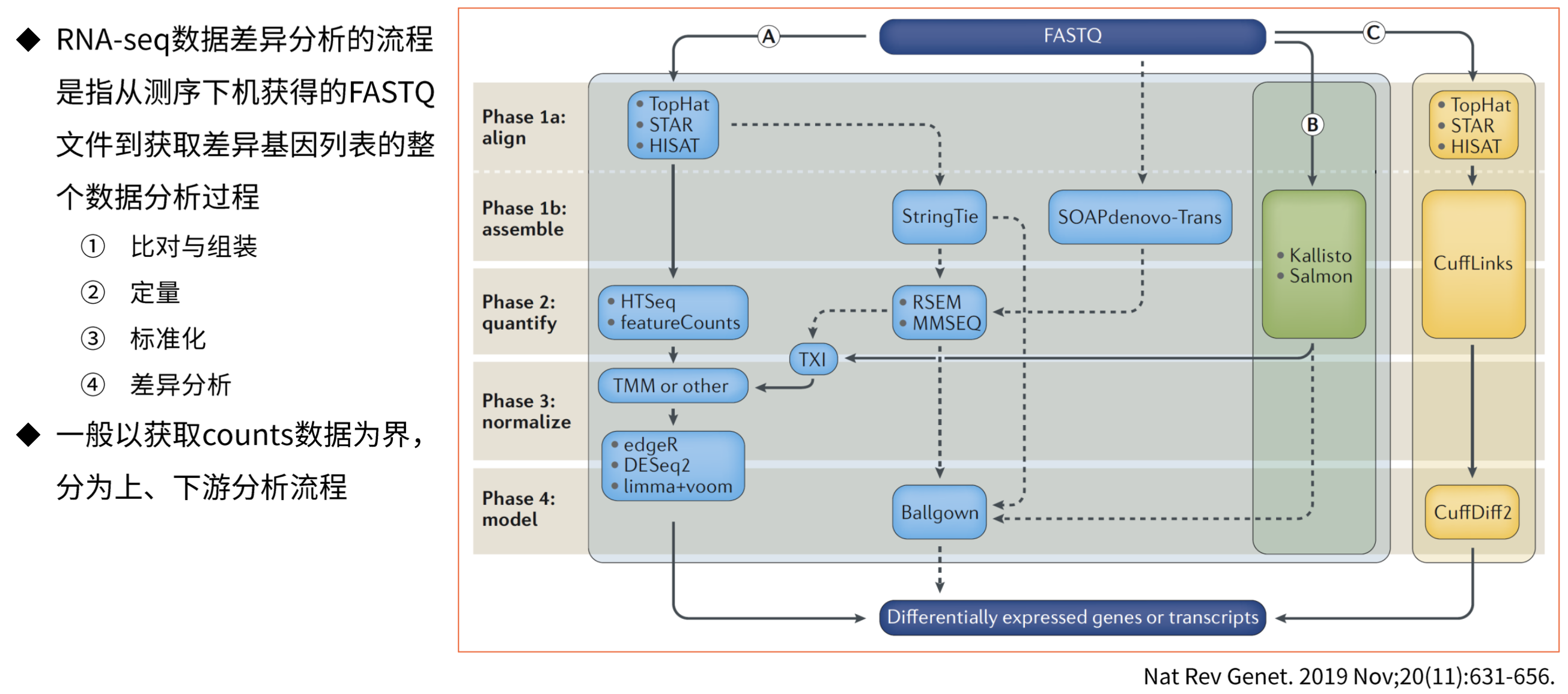
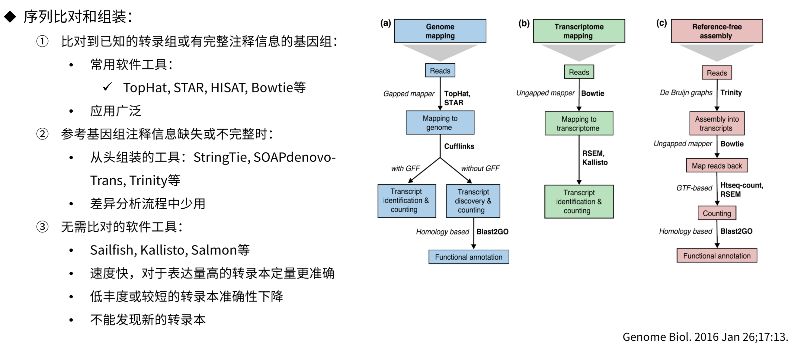
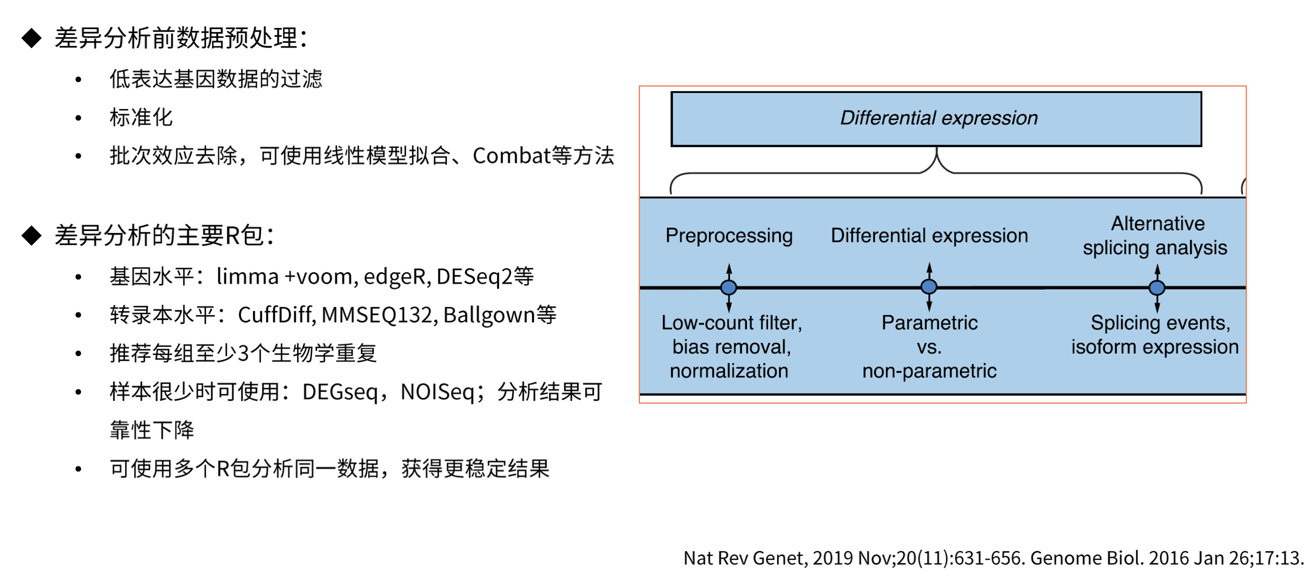
RNA-Seq分析流程
基因表达量数据类型
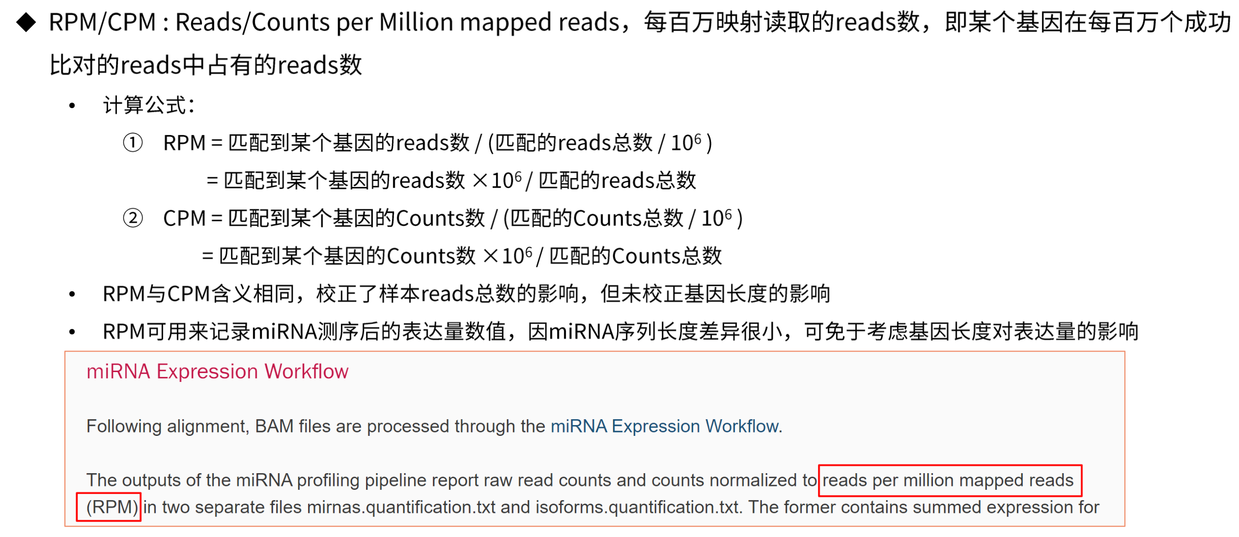
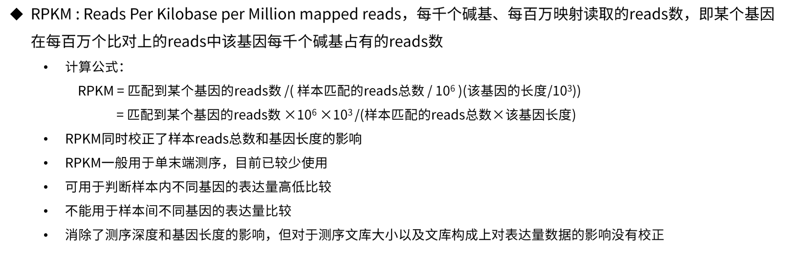
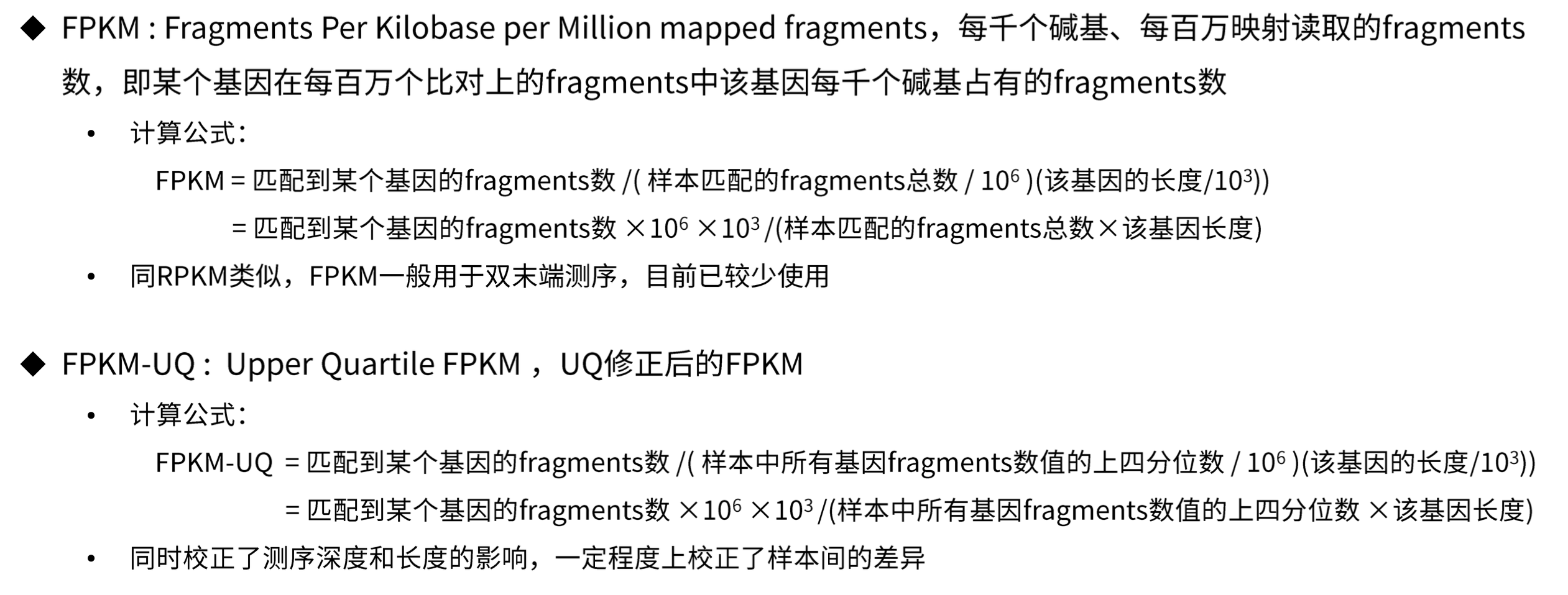
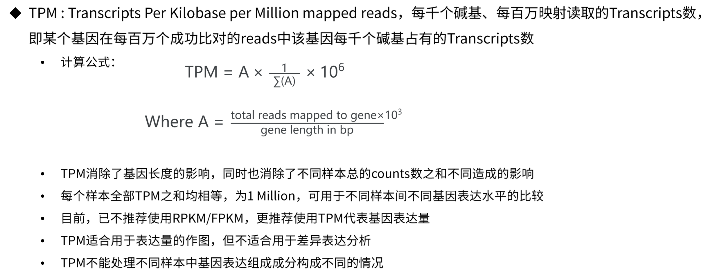
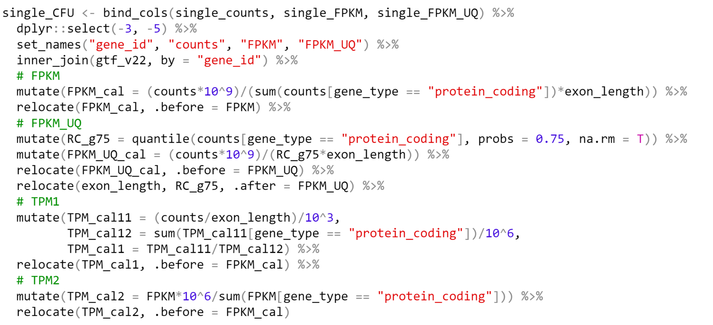
基因表达量数据转换
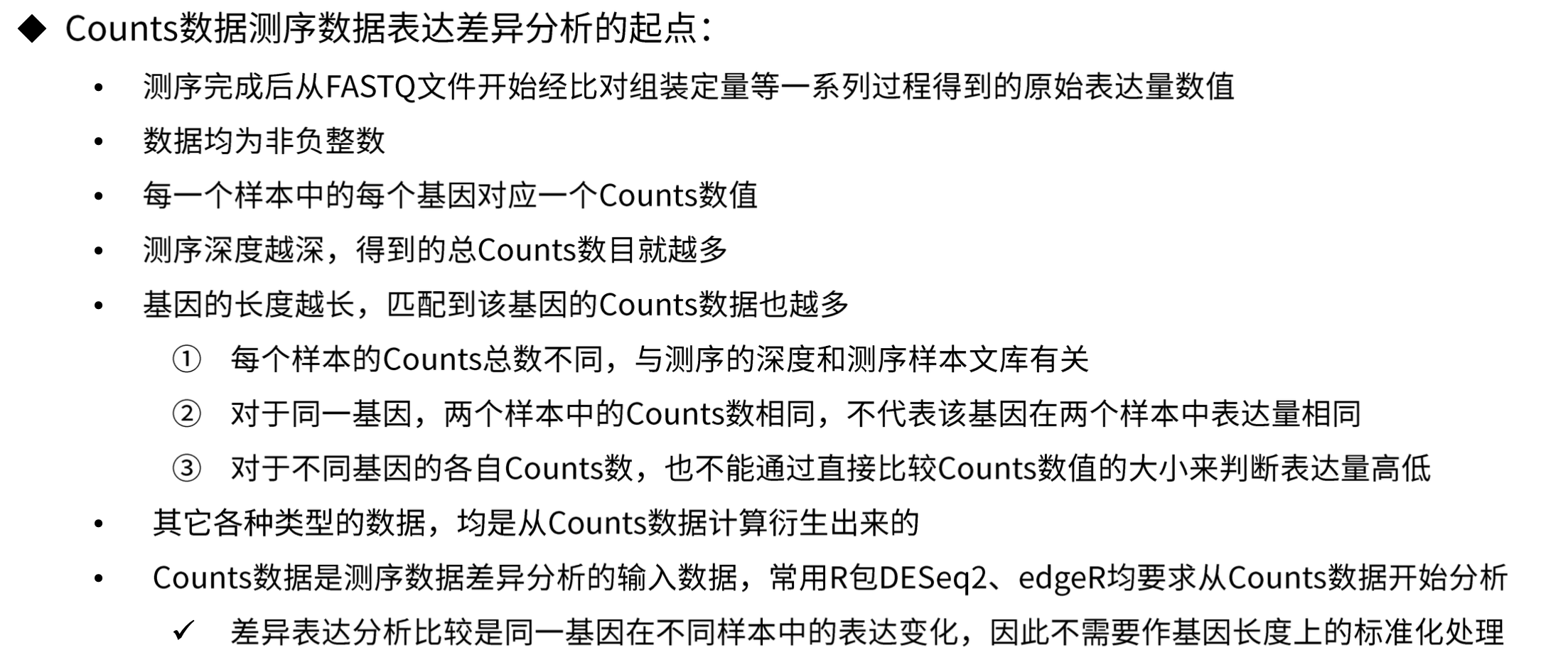
- 原始Counts数据
- 基因长度信息(外显子长度之和)
- 如按照protein-coding基因计算mapped reads计算,还需提供基因的分类信息